Note
Click here to download the full example code
Gradients and Spheres
This example shows how you can create gradient tables and sphere objects using DIPY_.
Usually, as we saw in example_quick_start, you load your b-values and b-vectors from disk and then you can create your own gradient table. But this time let’s say that you are an MR physicist and you want to design a new gradient scheme or you are a scientist who wants to simulate many different gradient schemes.
Now let’s assume that you are interested in creating a multi-shell acquisition with 2-shells, one at b=1000 \(s/mm^2\) and one at b=2500 \(s/mm^2\). For both shells let’s say that we want a specific number of gradients (64) and we want to have the points on the sphere evenly distributed.
This is possible using the disperse_charges which is an implementation of
electrostatic repulsion [Jones1999].
import numpy as np
from dipy.core.sphere import disperse_charges, Sphere, HemiSphere
We can first create some random points on a HemiSphere using spherical polar
coordinates.
n_pts = 64
theta = np.pi * np.random.rand(n_pts)
phi = 2 * np.pi * np.random.rand(n_pts)
hsph_initial = HemiSphere(theta=theta, phi=phi)
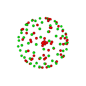
Next, we call disperse_charges which will iteratively move the points so that
the electrostatic potential energy is minimized.
hsph_updated, potential = disperse_charges(hsph_initial, 5000)
In hsph_updated we have the updated HemiSphere with the points nicely
distributed on the hemisphere. Let’s visualize them.
from dipy.viz import window, actor

# Enables/disables interactive visualization
interactive = False

scene = window.Scene()
scene.SetBackground(1, 1, 1)

scene.add(actor.point(hsph_initial.vertices, window.colors.red,
                      point_radius=0.05))
scene.add(actor.point(hsph_updated.vertices, window.colors.green,
                      point_radius=0.05))

print('Saving illustration as initial_vs_updated.png')
window.record(scene, out_path='initial_vs_updated.png', size=(300, 300))
if interactive:
    window.show(scene)
Saving illustration as initial_vs_updated.png

Illustration of electrostatic repulsion of red points which become green points.
We can also create a sphere from the hemisphere and show it in the following way.
sph = Sphere(xyz=np.vstack((hsph_updated.vertices, -hsph_updated.vertices)))

scene.clear()
scene.add(actor.point(sph.vertices, window.colors.green, point_radius=0.05))

print('Saving illustration as full_sphere.png')
window.record(scene, out_path='full_sphere.png', size=(300, 300))
if interactive:
    window.show(scene)
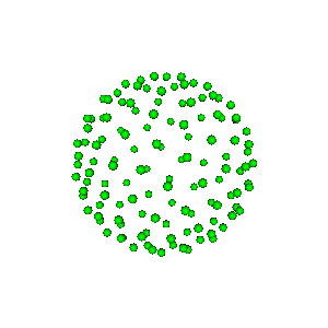
Saving illustration as full_sphere.png

It is time to create the Gradients. For this purpose we will use the
function gradient_table and fill it with the hsph_updated vectors that
we created above.
from dipy.core.gradients import gradient_table

vertices = hsph_updated.vertices
values = np.ones(vertices.shape[0])
We need two stacks of vertices, one for every shell, and we need two sets
of b-values, one at 1000 \(s/mm^2\), and one at 2500 \(s/mm^2\), as we discussed
previously.
bvecs = np.vstack((vertices, vertices))
bvals = np.hstack((1000 * values, 2500 * values))
We can also add some b0s. Let’s add one at the beginning and one at the end.
bvecs = np.insert(bvecs, (0, bvecs.shape[0]), np.array([0, 0, 0]), axis=0)
bvals = np.insert(bvals, (0, bvals.shape[0]), 0)

print(bvals)
[   0. 1000. 1000. 1000. 1000. 1000. 1000. 1000. 1000. 1000. 1000. 1000.
 1000. 1000. 1000. 1000. 1000. 1000. 1000. 1000. 1000. 1000. 1000. 1000.
 1000. 1000. 1000. 1000. 1000. 1000. 1000. 1000. 1000. 1000. 1000. 1000.
 1000. 1000. 1000. 1000. 1000. 1000. 1000. 1000. 1000. 1000. 1000. 1000.
 1000. 1000. 1000. 1000. 1000. 1000. 1000. 1000. 1000. 1000. 1000. 1000.
 1000. 1000. 1000. 1000. 1000. 2500. 2500. 2500. 2500. 2500. 2500. 2500.
 2500. 2500. 2500. 2500. 2500. 2500. 2500. 2500. 2500. 2500. 2500. 2500.
 2500. 2500. 2500. 2500. 2500. 2500. 2500. 2500. 2500. 2500. 2500. 2500.
 2500. 2500. 2500. 2500. 2500. 2500. 2500. 2500. 2500. 2500. 2500. 2500.
 2500. 2500. 2500. 2500. 2500. 2500. 2500. 2500. 2500. 2500. 2500. 2500.
 2500. 2500. 2500. 2500. 2500. 2500. 2500. 2500. 2500.    0.]
[    0.  1000.  1000.  1000.  1000.  1000.  1000.  1000.  1000.  1000.
  1000.  1000.  1000.  1000.  1000.  1000.  1000.  1000.  1000.  1000.
  1000.  1000.  1000.  1000.  1000.  1000.  1000.  1000.  1000.  1000.
  1000.  1000.  1000.  1000.  1000.  1000.  1000.  1000.  1000.  1000.
  1000.  1000.  1000.  1000.  1000.  1000.  1000.  1000.  1000.  1000.
  1000.  1000.  1000.  1000.  1000.  1000.  1000.  1000.  1000.  1000.
  1000.  1000.  1000.  1000.  1000.  2500.  2500.  2500.  2500.  2500.
  2500.  2500.  2500.  2500.  2500.  2500.  2500.  2500.  2500.  2500.
  2500.  2500.  2500.  2500.  2500.  2500.  2500.  2500.  2500.  2500.
  2500.  2500.  2500.  2500.  2500.  2500.  2500.  2500.  2500.  2500.
  2500.  2500.  2500.  2500.  2500.  2500.  2500.  2500.  2500.  2500.
  2500.  2500.  2500.  2500.  2500.  2500.  2500.  2500.  2500.  2500.
  2500.  2500.  2500.  2500.  2500.  2500.  2500.  2500.  2500.     0.]
print(bvecs)
[[ 0.          0.          0.        ]
 [ 0.48226551  0.8597359   0.16814924]
 [ 0.77169039  0.49362836  0.4010299 ]
 [ 0.91554673  0.21194055  0.34184117]
 [-0.7701603  -0.09150318  0.63125295]
 [-0.84451987  0.50221104  0.18593078]
 [-0.4654141  -0.57711311  0.67106644]
 [-0.07051484  0.19419914  0.97842442]
 [ 0.73214378  0.24406014  0.63592463]
 [-0.34081309  0.62007051  0.70665338]
 [-0.22612641 -0.05725387  0.97241392]
 [ 0.18986916  0.95549755  0.22577452]
 [ 0.92751189  0.36585046  0.07664942]
 [ 0.5401859  -0.41993756  0.72928159]
 [-0.58804797  0.4773355   0.65295513]
 [ 0.19614519  0.38822601  0.90044857]
 [ 0.62579607 -0.04787021  0.77851636]
 [ 0.92907407 -0.25474532  0.26819061]
 [-0.6961131  -0.55781155  0.45196552]
 [ 0.0728861  -0.76981131  0.63409634]
 [-0.97484953 -0.14227137  0.17154371]
 [-0.03030616 -0.99786452  0.05786142]
 [-0.42317947  0.88451485  0.1963482 ]
 [ 0.03669779 -0.21966671  0.97488451]
 [-0.10362895  0.49375687  0.86340326]
 [-0.8408654  -0.5135838   0.17081292]
 [-0.81009123  0.37987022  0.44659917]
 [-0.69068581  0.19345683  0.69679808]
 [-0.31272303 -0.34695196  0.88421075]
 [ 0.35300635 -0.66098507  0.66218219]
 [ 0.99363148  0.00729362  0.11244239]
 [ 0.52247988  0.72851389  0.44303756]
 [ 0.85807031 -0.02918715  0.5127021 ]
 [-0.10684707  0.95597749  0.27329605]
 [-0.08647343 -0.54092124  0.83661613]
 [ 0.5510663   0.50567611  0.66379033]
 [ 0.21428202  0.83939382  0.49950099]
 [ 0.21372546 -0.46400794  0.8596616 ]
 [ 0.84321252 -0.52227536  0.12736205]
 [-0.85972589 -0.29003618  0.42041694]
 [-0.50672214 -0.01651831  0.86195117]
 [-0.38505783  0.29286812  0.87519068]
 [-0.63196618 -0.76309358  0.13530312]
 [ 0.5407156  -0.82543672  0.16211372]
 [ 0.26638849 -0.9613867   0.06908539]
 [-0.59806911  0.6892814   0.40890647]
 [-0.96868622  0.22784374  0.09866226]
 [-0.33992264 -0.93389323  0.11088749]
 [ 0.76190618 -0.30103266  0.57347913]
 [-0.67816543  0.73063746  0.07912372]
 [ 0.50480845 -0.7455739   0.43507239]
 [-0.46054055 -0.79555927  0.39368497]
 [-0.12400492 -0.92299719  0.36427868]
 [ 0.22510718  0.06418008  0.97221791]
 [ 0.20641097 -0.90425752  0.37378182]
 [-0.60151254 -0.31767314  0.73298461]
 [-0.02649738  0.74745553  0.66378318]
 [ 0.74219636  0.65479978  0.14276492]
 [-0.28107091  0.82747339  0.48609354]
 [ 0.38166642 -0.18887159  0.90479736]
 [ 0.27396087  0.62529452  0.73072034]
 [ 0.72933698 -0.55231693  0.4037494 ]
 [-0.91454636  0.08554178  0.39533221]
 [-0.2293508  -0.74992219  0.6204957 ]
 [ 0.4754902   0.23790446  0.84694187]
 [ 0.          0.          0.        ]]
[[ 0.          0.          0.        ]
 [-0.80451777 -0.16877559  0.56944355]
 [ 0.32822557 -0.94355999  0.04430036]
 [-0.23584135 -0.96241331  0.13468285]
 [-0.39207424 -0.73505312  0.55314981]
 [-0.32539386 -0.16751384  0.93062235]
 [-0.82043195 -0.39411534  0.41420347]
 [ 0.65741493  0.74947875  0.07802061]
 [ 0.88853765  0.45303621  0.07251925]
 [ 0.39638642 -0.15185138  0.90543855]
                 ...
 [ 0.10175269  0.08197111  0.99142681]
 [ 0.50577702 -0.37862345  0.77513476]
 [ 0.42845026  0.40155296  0.80943535]
 [ 0.26939707  0.81103868  0.51927014]
 [-0.48938584 -0.43780086  0.75420946]
 [ 0.          0.          0.        ]]
Both b-values and b-vectors look correct. Let’s now create the
GradientTable.
gtab = gradient_table(bvals, bvecs)

scene.clear()
We can also visualize the gradients. Let’s color the first shell blue and the second shell cyan.
colors_b1000 = window.colors.blue * np.ones(vertices.shape)
colors_b2500 = window.colors.cyan * np.ones(vertices.shape)
colors = np.vstack((colors_b1000, colors_b2500))
colors = np.insert(colors, (0, colors.shape[0]), np.array([0, 0, 0]), axis=0)
colors = np.ascontiguousarray(colors)

scene.add(actor.point(gtab.gradients, colors, point_radius=100))

print('Saving illustration as gradients.png')
window.record(scene, out_path='gradients.png', size=(300, 300))
if interactive:
    window.show(scene)
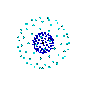
Saving illustration as gradients.png

References
Jones, DK. et al. Optimal strategies for measuring diffusion in anisotropic systems by magnetic resonance imaging, Magnetic Resonance in Medicine, vol 42, no 3, 515-525, 1999.
Total running time of the script: ( 0 minutes 2.568 seconds)