Reconstruct with Diffusion Spectrum Imaging

We show how to apply Diffusion Spectrum Imaging [Wedeen08] to diffusion MRI datasets of Cartesian keyhole diffusion gradients.

First import the necessary modules:

import numpy as np
from dipy.core.gradients import gradient_table
from dipy.data import get_fnames, get_sphere
from dipy.io.gradients import read_bvals_bvecs
from dipy.io.image import load_nifti
from dipy.reconst.dsi import DiffusionSpectrumModel

Download and get the data filenames for this tutorial.

fraw, fbval, fbvec = get_fnames('taiwan_ntu_dsi')

img contains a nibabel Nifti1Image object (data) and gtab contains a GradientTable object (gradient information e.g. b-values). For example to read the b-values it is possible to write print(gtab.bvals).

Load the raw diffusion data and the affine.

data, affine, voxel_size = load_nifti(fraw, return_voxsize=True)
bvals, bvecs = read_bvals_bvecs(fbval, fbvec)
bvecs[1:] = (bvecs[1:] /
                 np.sqrt(np.sum(bvecs[1:] * bvecs[1:], axis=1))[:, None])
gtab = gradient_table(bvals, bvecs)
print('data.shape (%d, %d, %d, %d)' % data.shape)

data.shape (96, 96, 60, 203)

data.shape (96, 96, 60, 203)

This dataset has anisotropic voxel sizes, therefore reslicing is necessary.

Instantiate the Model and apply it to the data.

dsmodel = DiffusionSpectrumModel(gtab)

Let’s just use one slice only from the data.

dataslice = data[:, :, data.shape[2] // 2]

dsfit = dsmodel.fit(dataslice)

  0%|          | 0/9216 [00:00<?, ?it/s]
100%|##########| 9216/9216 [00:00<00:00, 595622.45it/s]

Load an odf reconstruction sphere

sphere = get_sphere('repulsion724')

Calculate the ODFs with this specific sphere

ODF = dsfit.odf(sphere)

print('ODF.shape (%d, %d, %d)' % ODF.shape)

/Users/skoudoro/devel/dipy/dipy/reconst/dsi.py:173: RuntimeWarning: invalid value encountered in divide
  Pr /= Pr.sum()
ODF.shape (96, 96, 724)

ODF.shape (96, 96, 724)

In a similar fashion it is possible to calculate the PDFs of all voxels in one call with the following way

PDF = dsfit.pdf()

print('PDF.shape (%d, %d, %d, %d, %d)' % PDF.shape)

PDF.shape (96, 96, 17, 17, 17)

PDF.shape (96, 96, 17, 17, 17)

We see that even for a single slice this PDF array is close to 345 MBytes so we really have to be careful with memory usage when use this function with a full dataset.

The simple solution is to generate/analyze the ODFs/PDFs by iterating through each voxel and not store them in memory if that is not necessary.

from dipy.core.ndindex import ndindex

for index in ndindex(dataslice.shape[:2]):
    pdf = dsmodel.fit(dataslice[index]).pdf()

If you really want to save the PDFs of a full dataset on the disc we recommend using memory maps (numpy.memmap) but still have in mind that even if you do that for example for a dataset of volume size (96, 96, 60) you will need about 2.5 GBytes which can take less space when reasonable spheres (with < 1000 vertices) are used.

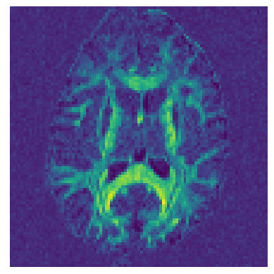
Let’s now calculate a map of Generalized Fractional Anisotropy (GFA) [Tuch04] using the DSI ODFs.

from dipy.reconst.odf import gfa

GFA = gfa(ODF)

import matplotlib.pyplot as plt

fig_hist, ax = plt.subplots(1)
ax.set_axis_off()
plt.imshow(GFA.T)
plt.savefig('dsi_gfa.png', bbox_inches='tight')

See also example_reconst_dsi_metrics for calculating different types of DSI maps.

Total running time of the script: ( 0 minutes 24.601 seconds)

Gallery generated by Sphinx-Gallery