Note
Click here to download the full example code
Mean signal diffusion kurtosis imaging (MSDKI)
Diffusion Kurtosis Imaging (DKI) is one of the conventional ways to estimate the degree of non-Gaussian diffusion (see example_reconst_dki) [Jensen2005]. However, a limitation of DKI is that its measures are highly sensitive to noise and image artefacts. For instance, due to the low radial diffusivities, standard kurtosis estimates in regions of well-aligned voxel may be corrupted by implausible low or even negative values.
A way to overcome this issue is to characterize kurtosis from average signals across all directions acquired for each data b-value (also known as powder-averaged signals). Moreover, as previously pointed [NetoHe2015], standard kurtosis measures (e.g. radial, axial and standard mean kurtosis) do not only depend on microstructural properties but also on mesoscopic properties such as fiber dispersion or the intersection angle of crossing fibers. In contrary, the kurtosis from powder-average signals has the advantage of not depending on the fiber distribution functions [NetoHe2018], [NetoHe2019].
In short, in this tutorial we show how to characterize non-Gaussian diffusion in a more precise way and decoupled from confounding effects of tissue dispersion and crossing.
In the first part of this example, we illustrate the properties of the measures obtained from the mean signal diffusion kurtosis imaging (MSDKI)[NetoHe2018]_ using synthetic data. Secondly, the mean signal diffusion kurtosis imaging will be applied to in-vivo MRI data. Finally, we show how MSDKI provides the same information than common microstructural models such as the spherical mean technique [NetoHe2019], [Kaden2016b].
Let’s import all relevant modules:
import numpy as np
import matplotlib.pyplot as plt

# Reconstruction modules
import dipy.reconst.dki as dki
import dipy.reconst.msdki as msdki

# For simulations
from dipy.sims.voxel import multi_tensor
from dipy.core.gradients import gradient_table
from dipy.core.sphere import disperse_charges, HemiSphere

# For in-vivo data
from dipy.data import get_fnames
from dipy.io.gradients import read_bvals_bvecs
from dipy.io.image import load_nifti
from dipy.segment.mask import median_otsu
Testing MSDKI in synthetic data
We simulate representative diffusion-weighted signals using MultiTensor simulations (for more information on this type of simulations see example_simulate_multi_tensor). For this example, simulations are produced based on the sum of four diffusion tensors to represent the intra- and extra-cellular spaces of two fiber populations. The parameters of these tensors are adjusted according to [NetoHe2015] (see also example_simulate_dki).
mevals = np.array([[0.00099, 0, 0],
                   [0.00226, 0.00087, 0.00087],
                   [0.00099, 0, 0],
                   [0.00226, 0.00087, 0.00087]])
For the acquisition parameters of the synthetic data, we use 60 gradient directions for two non-zero b-values (1000 and 2000 \(s/mm^{2}\)) and two zero bvalues (note that, such as the standard DKI, MSDKI requires at least three different b-values).
# Sample the spherical coordinates of 60 random diffusion-weighted directions.
n_pts = 60
theta = np.pi * np.random.rand(n_pts)
phi = 2 * np.pi * np.random.rand(n_pts)

# Convert direction to cartesian coordinates.
hsph_initial = HemiSphere(theta=theta, phi=phi)

# Evenly distribute the 60 directions
hsph_updated, potential = disperse_charges(hsph_initial, 5000)
directions = hsph_updated.vertices

# Reconstruct acquisition parameters for 2 non-zero=b-values and 2 b0s
bvals = np.hstack((np.zeros(2), 1000 * np.ones(n_pts), 2000 * np.ones(n_pts)))
bvecs = np.vstack((np.zeros((2, 3)), directions, directions))

gtab = gradient_table(bvals, bvecs)
Simulations are looped for different intra- and extra-cellular water volume fractions and different intersection angles of the two-fiber populations.
# Array containing the intra-cellular volume fractions tested
f = np.linspace(20, 80.0, num=7)

# Array containing the intersection angle
ang = np.linspace(0, 90.0, num=91)

# Matrix where synthetic signals will be stored
dwi = np.empty((f.size, ang.size, bvals.size))

for f_i in range(f.size):
    # estimating volume fractions for individual tensors
    fractions = np.array([100 - f[f_i], f[f_i], 100 - f[f_i], f[f_i]]) * 0.5

    for a_i in range(ang.size):
        # defining the directions for individual tensors
        angles = [(ang[a_i], 0.0), (ang[a_i], 0.0), (0.0, 0.0), (0.0, 0.0)]

        # producing signals using Dipy's function multi_tensor
        signal, sticks = multi_tensor(gtab, mevals, S0=100, angles=angles,
                                      fractions=fractions, snr=None)
        dwi[f_i, a_i, :] = signal
Now that all synthetic signals were produced, we can go forward with MSDKI fitting. As other Dipy’s reconstruction techniques, the MSDKI model has to be first defined for the specific GradientTable object of the synthetic data. For MSDKI, this is done by instantiating the MeanDiffusionKurtosisModel object in the following way:
msdki_model = msdki.MeanDiffusionKurtosisModel(gtab)
MSDKI can then be fitted to the synthetic data by calling the fit function
of this object:
msdki_fit = msdki_model.fit(dwi)
From the above fit object we can extract the two main parameters of the MSDKI, i.e.: 1) the mean signal diffusion (MSD); and 2) the mean signal kurtosis (MSK)
MSD = msdki_fit.msd
MSK = msdki_fit.msk
kurtosis (MK) from the standard DKI.
dki_model = dki.DiffusionKurtosisModel(gtab)
dki_fit = dki_model.fit(dwi)

MD = dki_fit.md
MK = dki_fit.mk(0, 3)
Now we plot the results as a function of the ground truth intersection angle and for different volume fractions of intra-cellular water.
fig1, axs = plt.subplots(nrows=2, ncols=2, figsize=(10, 10))

for f_i in range(f.size):
    axs[0, 0].plot(ang, MSD[f_i], linewidth=1.0,
                   label=':math:`F: %.2f`' % f[f_i])
    axs[0, 1].plot(ang, MSK[f_i], linewidth=1.0,
                   label=':math:`F: %.2f`' % f[f_i])
    axs[1, 0].plot(ang, MD[f_i], linewidth=1.0,
                   label=':math:`F: %.2f`' % f[f_i])
    axs[1, 1].plot(ang, MK[f_i], linewidth=1.0,
                   label=':math:`F: %.2f`' % f[f_i])

# Adjust properties of the first panel of the figure
axs[0, 0].set_xlabel('Intersection angle')
axs[0, 0].set_ylabel('MSD')
axs[0, 1].set_xlabel('Intersection angle')
axs[0, 1].set_ylabel('MSK')
axs[0, 1].legend(loc='center left', bbox_to_anchor=(1, 0.5))
axs[1, 0].set_xlabel('Intersection angle')
axs[1, 0].set_ylabel('MD')
axs[1, 1].set_xlabel('Intersection angle')
axs[1, 1].set_ylabel('MK')
axs[1, 1].legend(loc='center left', bbox_to_anchor=(1, 0.5))

plt.show()
fig1.savefig('MSDKI_simulations.png')
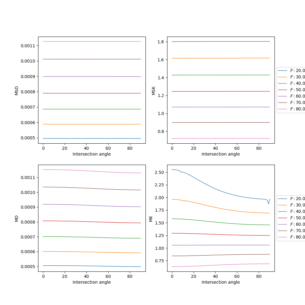

MSDKI and DKI measures for data of two crossing synthetic fibers. Upper panels show the MSDKI measures: 1) mean signal diffusivity (left panel); and 2) mean signal kurtosis (right panel). For reference, lower panels show the measures obtained by standard DKI: 1) mean diffusivity (left panel); and 2) mean kurtosis (right panel). All estimates are plotted as a function of the intersecting angle of the two crossing fibers. Different curves correspond to different ground truth axonal volume fraction of intra-cellular space.
The results of the above figure, demonstrate that both MSD and MSK are sensitive to axonal volume fraction (i.e. a microstructure property) but are independent to the intersection angle of the two crossing fibers (i.e. independent to properties regarding fiber orientation). In contrast, DKI measures seem to be independent to both axonal volume fraction and intersection angle.
Reconstructing diffusion data using MSDKI
Now that the properties of MSDKI were illustrated, let’s apply MSDKI to in-vivo diffusion-weighted data. As the example for the standard DKI (see example_reconst_dki), we use fetch to download a multi-shell dataset which was kindly provided by Hansen and Jespersen (more details about the data are provided in their paper [Hansen2016]). The total size of the downloaded data is 192 MBytes, however you only need to fetch it once.
fraw, fbval, fbvec, t1_fname = get_fnames('cfin_multib')

data, affine = load_nifti(fraw)
bvals, bvecs = read_bvals_bvecs(fbval, fbvec)
gtab = gradient_table(bvals, bvecs)
Before fitting the data, we perform some data pre-processing. For illustration, we only mask the data to avoid unnecessary calculations on the background of the image; however, you could also apply other pre-processing techniques. For example, some state of the art denoising algorithms are available in DIPY_ (e.g. the non-local means filter example-denoise-nlmeans or the local pca example-denoise-localpca).
maskdata, mask = median_otsu(data, vol_idx=[0, 1], median_radius=4, numpass=2,
                             autocrop=False, dilate=1)
Now that we have loaded and pre-processed the data we can go forward with MSDKI fitting. As for the synthetic data, the MSDKI model has to be first defined for the data’s GradientTable object:
msdki_model = msdki.MeanDiffusionKurtosisModel(gtab)
The data can then be fitted by calling the fit function of this object:
msdki_fit = msdki_model.fit(data, mask=mask)
Let’s then extract the two main MSDKI’s parameters: 1) mean signal diffusion (MSD); and 2) mean signal kurtosis (MSK).
MSD = msdki_fit.msd
MSK = msdki_fit.msk
For comparison, we calculate also the mean diffusivity (MD) and mean kurtosis (MK) from the standard DKI.
dki_model = dki.DiffusionKurtosisModel(gtab)
dki_fit = dki_model.fit(data, mask=mask)

MD = dki_fit.md
MK = dki_fit.mk(0, 3)
Let’s now visualize the data using matplotlib for a selected axial slice.
axial_slice = 9

fig2, ax = plt.subplots(2, 2, figsize=(6, 6),
                        subplot_kw={'xticks': [], 'yticks': []})

fig2.subplots_adjust(hspace=0.3, wspace=0.05)

im0 = ax.flat[0].imshow(MSD[:, :, axial_slice].T * 1000, cmap='gray',
                        vmin=0, vmax=2, origin='lower')
ax.flat[0].set_title('MSD (MSDKI)')

im1 = ax.flat[1].imshow(MSK[:, :, axial_slice].T, cmap='gray',
                        vmin=0, vmax=2, origin='lower')
ax.flat[1].set_title('MSK (MSDKI)')

im2 = ax.flat[2].imshow(MD[:, :, axial_slice].T * 1000, cmap='gray',
                        vmin=0, vmax=2, origin='lower')
ax.flat[2].set_title('MD (DKI)')

im3 = ax.flat[3].imshow(MK[:, :, axial_slice].T, cmap='gray',
                        vmin=0, vmax=2, origin='lower')
ax.flat[3].set_title('MK (DKI)')

fig2.colorbar(im0, ax=ax.flat[0])
fig2.colorbar(im1, ax=ax.flat[1])
fig2.colorbar(im2, ax=ax.flat[2])
fig2.colorbar(im3, ax=ax.flat[3])

plt.show()
fig2.savefig('MSDKI_invivo.png')
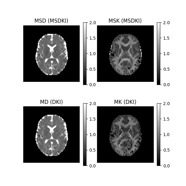
This figure shows that the contrast of in-vivo MSD and MSK maps (upper panels) are similar to the contrast of MD and MSK maps (lower panels); however, in the upper part we insure that direct contributions of fiber dispersion were removed. The upper panels also reveal that MSDKI measures are let sensitive to noise artefacts than standard DKI measures (as pointed by [NetoHe2018]), particularly one can observe that MSK maps always present positive values in brain white matter regions, while implausible negative kurtosis values are present in the MK maps in the same regions.
Relationship between MSDKI and SMT2
As showed in [NetoHe2019], MSDKI captures the same information than the spherical mean technique (SMT) microstructural models [Kaden2016b]. In this way, the SMT model parameters can be directly computed from MSDKI. For instance, the axonal volume fraction (f), the intrisic diffusivity (di), and the microscopic anisotropy of the SMT 2-compartmental model [NetoHe2019] can be extracted using the following lines of code:
F = msdki_fit.smt2f
DI = msdki_fit.smt2di
uFA2 = msdki_fit.smt2uFA
fig3, ax = plt.subplots(1, 3, figsize=(9, 2.5),
                        subplot_kw={'xticks': [], 'yticks': []})

fig3.subplots_adjust(hspace=0.4, wspace=0.1)

im0 = ax.flat[0].imshow(F[:, :, axial_slice].T,
                        cmap='gray', vmin=0, vmax=1, origin='lower')
ax.flat[0].set_title('SMT2 f (MSDKI)')

im1 = ax.flat[1].imshow(DI[:, :, axial_slice].T * 1000, cmap='gray',
                        vmin=0, vmax=2, origin='lower')
ax.flat[1].set_title('SMT2 di (MSDKI)')

im2 = ax.flat[2].imshow(uFA2[:, :, axial_slice].T, cmap='gray',
                        vmin=0, vmax=1, origin='lower')
ax.flat[2].set_title('SMT2 uFA (MSDKI)')

fig3.colorbar(im0, ax=ax.flat[0])
fig3.colorbar(im1, ax=ax.flat[1])
fig3.colorbar(im2, ax=ax.flat[2])


plt.show()
fig3.savefig('MSDKI_SMT2_invivo.png')
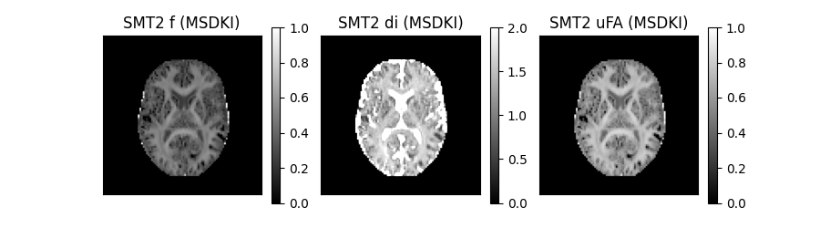
The similar contrast of SMT2 f-parameter maps in comparison to MSK (first panel of Figure 3 vs second panel of Figure 2) confirms than MSK and F captures the same tissue information but on different scales (but rescaled to values between 0 and 1). It is important to note that SMT model parameters estimates should be used with care, because the SMT model was shown to be invalid NetoHe2019]_. For instance, although SMT2 parameter f and uFA may be a useful normalization of the degree of non-Gaussian diffusion (note than both metrics have a range between 0 and 1), these cannot be interpreted as a real biophysical estimates of axonal water fraction and tissue microscopic anisotropy.
References
Jensen JH, Helpern JA, Ramani A, Lu H, Kaczynski K (2005). Diffusional Kurtosis Imaging: The Quantification of Non_Gaussian Water Diffusion by Means of Magnetic Resonance Imaging. Magnetic Resonance in Medicine 53: 1432-1440
Neto Henriques R, Correia MM, Nunes RG, Ferreira HA (2015). Exploring the 3D geometry of the diffusion kurtosis tensor - Impact on the development of robust tractography procedures and novel biomarkers, NeuroImage 111: 85-99
Henriques RN, 2018. Advanced Methods for Diffusion MRI Data Analysis and their Application to the Healthy Ageing Brain (Doctoral thesis). Downing College, University of Cambridge. https://doi.org/10.17863/CAM.29356
Neto Henriques R, Jespersen SN, Shemesh N (2019). Microscopic anisotropy misestimation in spherical‐mean single diffusion encoding MRI. Magnetic Resonance in Medicine (In press). doi: 10.1002/mrm.27606
Kaden E, Kelm ND, Carson RP, Does MD, Alexander DC (2016) Multi-compartment microscopic diffusion imaging. NeuroImage 139: 346-359.
Hansen, B, Jespersen, SN (2016). Data for evaluation of fast kurtosis strategies, b-value optimization and exploration of diffusion MRI contrast. Scientific Data 3: 160072 doi:10.1038/sdata.2016.72
Total running time of the script: ( 3 minutes 57.870 seconds)