Note
Click here to download the full example code
Calculate SHORE scalar maps
We show how to calculate two SHORE-based scalar maps: return to origin probability (RTOP) [Descoteaux2011] and mean square displacement (MSD) [Wu2007], [Wu2008] on your data. SHORE can be used with any multiple b-value dataset like multi-shell or DSI.
First import the necessary modules:
import numpy as np
import matplotlib.pyplot as plt
from dipy.core.gradients import gradient_table
from dipy.data import get_fnames
from dipy.io.gradients import read_bvals_bvecs
from dipy.io.image import load_nifti
from dipy.reconst.shore import ShoreModel
Download and get the data filenames for this tutorial.
fraw, fbval, fbvec = get_fnames('taiwan_ntu_dsi')
img contains a nibabel Nifti1Image object (data) and gtab contains a GradientTable object (gradient information e.g. b-values). For example, to read the b-values it is possible to write print(gtab.bvals).
Load the raw diffusion data and the affine.
data, affine = load_nifti(fraw)
bvals, bvecs = read_bvals_bvecs(fbval, fbvec)
bvecs[1:] = (bvecs[1:] /
             np.sqrt(np.sum(bvecs[1:] * bvecs[1:], axis=1))[:, None])
gtab = gradient_table(bvals, bvecs)
print('data.shape (%d, %d, %d, %d)' % data.shape)
data.shape (96, 96, 60, 203)
Instantiate the Model.
asm = ShoreModel(gtab)
Let’s just use only one slice only from the data.
dataslice = data[30:70, 20:80, data.shape[2] // 2]
Fit the signal with the model and calculate the SHORE coefficients.
asmfit = asm.fit(dataslice)
  0%|          | 0/2400 [00:00<?, ?it/s]
 10%|#         | 244/2400 [00:00<00:00, 2434.25it/s]
 21%|##1       | 504/2400 [00:00<00:00, 2526.83it/s]
 32%|###1      | 766/2400 [00:00<00:00, 2567.48it/s]
 43%|####3     | 1043/2400 [00:00<00:00, 2646.80it/s]
 55%|#####4    | 1308/2400 [00:00<00:00, 2581.71it/s]
 65%|######5   | 1567/2400 [00:00<00:00, 2580.23it/s]
 76%|#######6  | 1828/2400 [00:00<00:00, 2589.56it/s]
 87%|########7 | 2094/2400 [00:00<00:00, 2610.44it/s]
 98%|#########8| 2363/2400 [00:00<00:00, 2633.67it/s]
100%|##########| 2400/2400 [00:00<00:00, 2597.90it/s]
Calculate the analytical RTOP on the signal that corresponds to the integral of the signal.
print('Calculating... rtop_signal')
rtop_signal = asmfit.rtop_signal()
Calculating... rtop_signal
Now we calculate the analytical RTOP on the propagator, that corresponds to its central value.
print('Calculating... rtop_pdf')
rtop_pdf = asmfit.rtop_pdf()
Calculating... rtop_pdf
In theory, these two measures must be equal, to show that we calculate the mean square error on this two measures.
mse = np.sum((rtop_signal - rtop_pdf) ** 2) / rtop_signal.size
print("MSE = %f" % mse)
MSE = 0.000000
MSE = 0.000000
Let’s calculate the analytical mean square displacement on the propagator.
print('Calculating... msd')
msd = asmfit.msd()
Calculating... msd
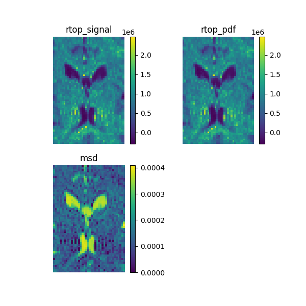
Show the maps and save them to a file.
fig = plt.figure(figsize=(6, 6))
ax1 = fig.add_subplot(2, 2, 1, title='rtop_signal')
ax1.set_axis_off()
ind = ax1.imshow(rtop_signal.T, interpolation='nearest', origin='lower')
plt.colorbar(ind)
ax2 = fig.add_subplot(2, 2, 2, title='rtop_pdf')
ax2.set_axis_off()
ind = ax2.imshow(rtop_pdf.T, interpolation='nearest', origin='lower')
plt.colorbar(ind)
ax3 = fig.add_subplot(2, 2, 3, title='msd')
ax3.set_axis_off()
ind = ax3.imshow(msd.T, interpolation='nearest', origin='lower', vmin=0)
plt.colorbar(ind)
plt.savefig('SHORE_maps.png')

References
Descoteaux M. et al., “Multiple q-shell diffusion propagator imaging”, Medical Image Analysis, vol 15, No. 4, p. 603-621, 2011.
Wu Y. et al., “Hybrid diffusion imaging”, NeuroImage, vol 36, p. 617-629, 2007.
Wu Y. et al., “Computation of Diffusion Function Measures in q-Space Using Magnetic Resonance Hybrid Diffusion Imaging”, IEEE TRANSACTIONS ON MEDICAL IMAGING, vol. 27, No. 6, p. 858-865, 2008.
Total running time of the script: ( 0 minutes 2.959 seconds)