Note
Click here to download the full example code
Denoise images using the Marcenko-Pastur PCA algorithm
The PCA-based denoising algorithm exploits the redundancy across the diffusion-weighted images [Manjon2013], [Veraart2016a]. This algorithm has been shown to provide an optimal compromise between noise suppression and loss of anatomical information for different techniques such as DTI [Manjon2013], spherical deconvolution [Veraart2016a] and DKI [Henri2018].
The basic idea behind the PCA-based denoising algorithms is to remove the components of the data that are classified as noise. The Principal Components classification can be performed based on prior noise variance estimates [Manjon2013] (see denoise_localpca) or automatically based on the Marcenko-Pastur distribution [Veraa2016a]. In addition to noise suppression, the PCA algorithm can be used to get the standard deviation of the noise [Veraa2016b].
In the following example, we show how to denoise diffusion MRI images and estimate the noise standard deviation using the PCA algorithm based on the Marcenko-Pastur distribution [Veraa2016a]
Let’s load the necessary modules
# load general modules
import numpy as np
import nibabel as nib
import matplotlib.pyplot as plt
from time import time

# load main pca function using Marcenko-Pastur distribution
from dipy.denoise.localpca import mppca

# load functions to fetch data for this example
from dipy.data import get_fnames

# load other dipy's functions that will be used for auxiliary analysis
from dipy.core.gradients import gradient_table
from dipy.io.image import load_nifti
from dipy.io.gradients import read_bvals_bvecs
from dipy.segment.mask import median_otsu
import dipy.reconst.dki as dki
For this example, we use fetch to download a multi-shell dataset which was kindly provided by Hansen and Jespersen (more details about the data are provided in their paper [Hansen2016]). The total size of the downloaded data is 192 MBytes, however you only need to fetch it once.
dwi_fname, dwi_bval_fname, dwi_bvec_fname, _ = get_fnames('cfin_multib')
data, affine = load_nifti(dwi_fname)
bvals, bvecs = read_bvals_bvecs(dwi_bval_fname, dwi_bvec_fname)
gtab = gradient_table(bvals, bvecs)
For the sake of simplicity, we only select two non-zero b-values for this example.
bvals = gtab.bvals

bvecs = gtab.bvecs

sel_b = np.logical_or(np.logical_or(bvals == 0, bvals == 1000), bvals == 2000)

data = data[..., sel_b]

gtab = gradient_table(bvals[sel_b], bvecs[sel_b])

print(data.shape)
(96, 96, 19, 67)
As one can see from its shape, the selected data contains a total of 67 volumes of images corresponding to all the diffusion gradient directions of the selected b-values.
The PCA denoising using the Marcenko-Pastur distribution can be performed by
calling the function mppca:
t = time()

denoised_arr = mppca(data, patch_radius=2)

print("Time taken for local MP-PCA ", -t + time())
Time taken for local MP-PCA 637.1518270969391
Internally, the mppca algorithm denoises the diffusion-weighted data
using a 3D sliding window which is defined by the variable patch_radius.
In total, this window should comprise a larger number of voxels than the number
of diffusion-weighted volumes. Since our data has a total of 67 volumes, the
patch_radius is set to 2 which corresponds to a 5x5x5 sliding window
comprising a total of 125 voxels.
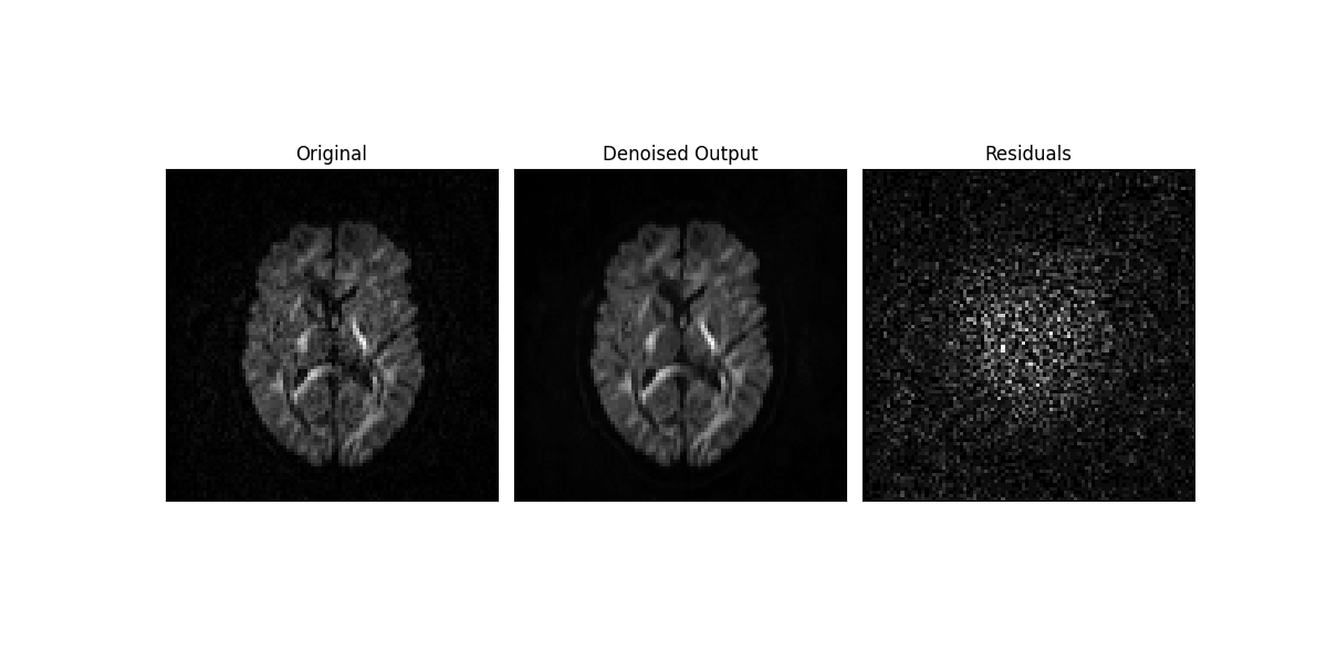
To assess the performance of the Marcenko-Pastur PCA denoising algorithm, an axial slice of the original data, denoised data, and residuals are plotted below:
sli = data.shape[2] // 2
gra = data.shape[3] - 1
orig = data[:, :, sli, gra]
den = denoised_arr[:, :, sli, gra]
rms_diff = np.sqrt((orig - den) ** 2)

fig1, ax = plt.subplots(1, 3, figsize=(12, 6),
                        subplot_kw={'xticks': [], 'yticks': []})

fig1.subplots_adjust(hspace=0.3, wspace=0.05)

ax.flat[0].imshow(orig.T, cmap='gray', interpolation='none',
                  origin='lower')
ax.flat[0].set_title('Original')
ax.flat[1].imshow(den.T, cmap='gray', interpolation='none',
                  origin='lower')
ax.flat[1].set_title('Denoised Output')
ax.flat[2].imshow(rms_diff.T, cmap='gray', interpolation='none',
                  origin='lower')
ax.flat[2].set_title('Residuals')

fig1.savefig('denoised_mppca.png')

print("The result saved in denoised_mppca.png")
The result saved in denoised_mppca.png

The noise suppression can be visually appreciated by comparing the original data slice (left panel) to its denoised version (middle panel). The difference between original and denoised data showing only random noise indicates that the data’s structural information is preserved by the PCA denoising algorithm (right panel).
Below we show how the denoised data can be saved.
nib.save(nib.Nifti1Image(denoised_arr,
                         affine), 'denoised_mppca.nii.gz')

print("Entire denoised data saved in denoised_mppca.nii.gz")
Entire denoised data saved in denoised_mppca.nii.gz
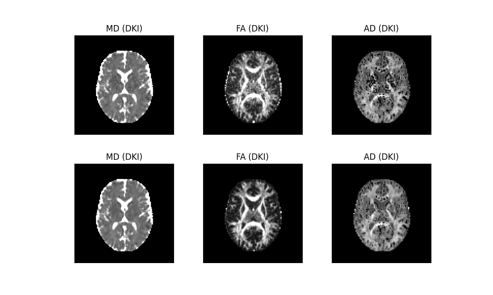
Additionally, we show how the PCA denoising algorithm affects different diffusion measurements. For this, we run the diffusion kurtosis model below on both original and denoised versions of the data:
dkimodel = dki.DiffusionKurtosisModel(gtab)

maskdata, mask = median_otsu(data, vol_idx=[0, 1], median_radius=4, numpass=2,
                             autocrop=False, dilate=1)

dki_orig = dkimodel.fit(data, mask=mask)
dki_den = dkimodel.fit(denoised_arr, mask=mask)
We use the following code to plot the MD, FA and MK estimates from the two data fits:
FA_orig = dki_orig.fa
FA_den = dki_den.fa
MD_orig = dki_orig.md
MD_den = dki_den.md
MK_orig = dki_orig.mk(0, 3)
MK_den = dki_den.mk(0, 3)


fig2, ax = plt.subplots(2, 3, figsize=(10, 6),
                        subplot_kw={'xticks': [], 'yticks': []})

fig2.subplots_adjust(hspace=0.3, wspace=0.03)

ax.flat[0].imshow(MD_orig[:, :, sli].T, cmap='gray', vmin=0, vmax=2.0e-3,
                  origin='lower')
ax.flat[0].set_title('MD (DKI)')
ax.flat[1].imshow(FA_orig[:, :, sli].T, cmap='gray', vmin=0, vmax=0.7,
                  origin='lower')
ax.flat[1].set_title('FA (DKI)')
ax.flat[2].imshow(MK_orig[:, :, sli].T, cmap='gray', vmin=0, vmax=1.5,
                  origin='lower')
ax.flat[2].set_title('AD (DKI)')
ax.flat[3].imshow(MD_den[:, :, sli].T, cmap='gray', vmin=0, vmax=2.0e-3,
                  origin='lower')
ax.flat[3].set_title('MD (DKI)')
ax.flat[4].imshow(FA_den[:, :, sli].T, cmap='gray', vmin=0, vmax=0.7,
                  origin='lower')
ax.flat[4].set_title('FA (DKI)')
ax.flat[5].imshow(MK_den[:, :, sli].T, cmap='gray', vmin=0, vmax=1.5,
                  origin='lower')
ax.flat[5].set_title('AD (DKI)')
plt.show()
fig2.savefig('denoised_dki.png')

print("The result saved in denoised_dki.png")
The result saved in denoised_dki.png

In the above figure, the DKI maps obtained from the original data are shown in the upper panels, while the DKI maps from the denoised data are shown in the lower panels. Substantial improvements in measurement robustness can be visually appreciated, particularly for the FA and MK estimates.
Noise standard deviation estimation using the Marcenko-Pastur PCA algorithm
As mentioned above, the Marcenko-Pastur PCA algorithm can also be used to
estimate the image’s noise standard deviation (std). The noise std
automatically computed from the mppca function can be returned by
setting the optional input parameter return_sigma to True.
denoised_arr, sigma = mppca(data, patch_radius=2, return_sigma=True)
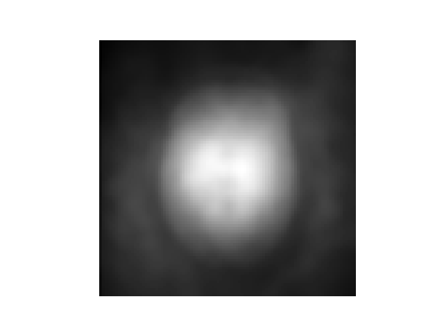
Let’s plot the noise standard deviation estimate:
fig3 = plt.figure('PCA Noise standard deviation estimation')
plt.imshow(sigma[..., sli].T, cmap='gray', origin='lower')
plt.axis('off')
plt.show()
fig3.savefig('pca_sigma.png')

print("The result saved in pca_sigma.png")
The result saved in pca_sigma.png

The above figure shows that the Marcenko-Pastur PCA algorithm computes a 3D spatial varying noise level map. To obtain the mean noise std across all voxels, you can use the following lines of code:
mean_sigma = np.mean(sigma[mask])

print(mean_sigma)
4.6833844
Below we use this mean noise level estimate to compute the nominal SNR of the data (i.e. SNR at b-value=0):
b0 = denoised_arr[..., 0]

mean_signal = np.mean(b0[mask])

snr = mean_signal / mean_sigma

print(snr)
34.56180377412377
References
Manjon JV, Coupe P, Concha L, Buades A, Collins DL “Diffusion Weighted Image Denoising Using Overcomplete Local PCA” (2013). PLoS ONE 8(9): e73021. doi:10.1371/journal.pone.0073021.
Veraart J, Fieremans E, Novikov DS. 2016. Diffusion MRI noise mapping using random matrix theory. Magnetic Resonance in Medicine. doi: 10.1002/mrm.26059.
Henriques, R., 2018. Advanced Methods for Diffusion MRI Data Analysis and their Application to the Healthy Ageing Brain (Doctoral thesis). https://doi.org/10.17863/CAM.29356
Veraart J, Novikov DS, Christiaens D, Ades-aron B, Sijbers, Fieremans E, 2016. Denoising of Diffusion MRI using random matrix theory. Neuroimage 142:394-406. doi: 10.1016/j.neuroimage.2016.08.016
Total running time of the script: ( 21 minutes 54.002 seconds)