Note
Click here to download the full example code
SNR estimation for Diffusion-Weighted Images
Computing the Signal-to-Noise-Ratio (SNR) of DW images is still an open question, as SNR depends on the white matter structure of interest as well as the gradient direction corresponding to each DWI.
In classical MRI, SNR can be defined as the ratio of the mean of the signal divided by the standard deviation of the underlying Gaussian noise, that is \(SNR = mean(signal) / std(noise)\). The noise standard deviation can be computed from the background in any of the DW images. How do we compute the mean of the signal, and what signal?
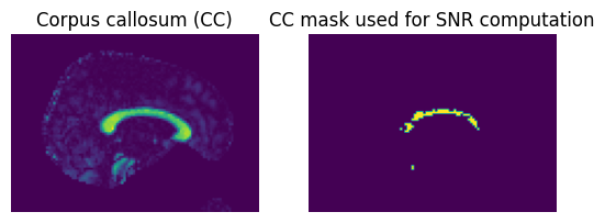
The strategy here is to compute a ‘worst-case’ SNR for DWI. Several white matter structures such as the corpus callosum (CC), corticospinal tract (CST), or the superior longitudinal fasciculus (SLF) can be easily identified from the colored-FA (CFA) map. In this example, we will use voxels from the CC, which have the characteristic of being highly red in the CFA map since they are mainly oriented in the left-right direction. We know that the DW image closest to the X-direction will be the one with the most attenuated diffusion signal. This is the strategy adopted in several recent papers (see [Descoteaux2011] and [Jones2013]). It gives a good indication of the quality of the DWI data.
First, we compute the tensor model in a brain mask (see the Reconstruction of the diffusion signal with the Tensor model example for further explanations).
import numpy as np
from dipy.core.gradients import gradient_table
from dipy.data import get_fnames
from dipy.io.gradients import read_bvals_bvecs
from dipy.io.image import load_nifti, save_nifti
from dipy.segment.mask import median_otsu
from dipy.reconst.dti import TensorModel

hardi_fname, hardi_bval_fname, hardi_bvec_fname = get_fnames('stanford_hardi')

data, affine = load_nifti(hardi_fname)
bvals, bvecs = read_bvals_bvecs(hardi_bval_fname, hardi_bvec_fname)
gtab = gradient_table(bvals, bvecs)

print('Computing brain mask...')
b0_mask, mask = median_otsu(data, vol_idx=[0])

print('Computing tensors...')
tenmodel = TensorModel(gtab)
tensorfit = tenmodel.fit(data, mask=mask)
Computing brain mask...
Computing tensors...
Next, we set our red-green-blue thresholds to (0.6, 1) in the x axis and (0, 0.1) in the y and z axes respectively. These values work well in practice to isolate the very RED voxels of the cfa map.
Then, as assurance, we want just RED voxels in the CC (there could be noisy red voxels around the brain mask and we don’t want those). Unless the brain acquisition was badly aligned, the CC is always close to the mid-sagittal slice.
The following lines perform these two operations and then saves the computed mask.
print('Computing worst-case/best-case SNR using the corpus callosum...')
from dipy.segment.mask import segment_from_cfa
from dipy.segment.mask import bounding_box

threshold = (0.6, 1, 0, 0.1, 0, 0.1)
CC_box = np.zeros_like(data[..., 0])

mins, maxs = bounding_box(mask)
mins = np.array(mins)
maxs = np.array(maxs)
diff = (maxs - mins) // 4
bounds_min = mins + diff
bounds_max = maxs - diff

CC_box[bounds_min[0]:bounds_max[0],
       bounds_min[1]:bounds_max[1],
       bounds_min[2]:bounds_max[2]] = 1

mask_cc_part, cfa = segment_from_cfa(tensorfit, CC_box, threshold,
                                     return_cfa=True)

save_nifti('cfa_CC_part.nii.gz', (cfa*255).astype(np.uint8), affine)
save_nifti('mask_CC_part.nii.gz', mask_cc_part.astype(np.uint8), affine)

import matplotlib.pyplot as plt
region = 40
fig = plt.figure('Corpus callosum segmentation')
plt.subplot(1, 2, 1)
plt.title("Corpus callosum (CC)")
plt.axis('off')
red = cfa[..., 0]
plt.imshow(np.rot90(red[region, ...]))

plt.subplot(1, 2, 2)
plt.title("CC mask used for SNR computation")
plt.axis('off')
plt.imshow(np.rot90(mask_cc_part[region, ...]))
fig.savefig("CC_segmentation.png", bbox_inches='tight')
Computing worst-case/best-case SNR using the corpus callosum...

x-direction, we can use all the voxels to estimate the mean signal in this region.
mean_signal = np.mean(data[mask_cc_part], axis=0)
computed before and invert it to catch the outside of the brain. This could also be determined manually with a ROI in the background. [Warning: Certain MR manufacturers mask out the outside of the brain with 0’s. One thus has to be careful how the noise ROI is defined].
from scipy.ndimage import binary_dilation
mask_noise = binary_dilation(mask, iterations=10)
mask_noise[..., :mask_noise.shape[-1]//2] = 1
mask_noise = ~mask_noise

save_nifti('mask_noise.nii.gz', mask_noise.astype(np.uint8), affine)

noise_std = np.std(data[mask_noise, :])
print('Noise standard deviation sigma= ', noise_std)
Noise standard deviation sigma= 8.17113266785504
for DW images with gradient direction that lies the closest to the X, Y and Z axes.
# Exclude null bvecs from the search
idx = np.sum(gtab.bvecs, axis=-1) == 0
gtab.bvecs[idx] = np.inf
axis_X = np.argmin(np.sum((gtab.bvecs-np.array([1, 0, 0]))**2, axis=-1))
axis_Y = np.argmin(np.sum((gtab.bvecs-np.array([0, 1, 0]))**2, axis=-1))
axis_Z = np.argmin(np.sum((gtab.bvecs-np.array([0, 0, 1]))**2, axis=-1))

for direction in [0, axis_X, axis_Y, axis_Z]:
    SNR = mean_signal[direction]/noise_std
    if direction == 0:
        print("SNR for the b=0 image is :", SNR)
    else:
        print("SNR for direction", direction, " ",
              gtab.bvecs[direction], "is :", SNR)
SNR for the b=0 image is : 47.366354266706736
SNR for direction 58   [ 0.98875  0.1177  -0.09229] is : 5.918432129721111
SNR for direction 57   [-0.05039    0.99871    0.0054406] is : 26.72068171809924
SNR for direction 126   [-0.11825  -0.039925  0.99218 ] is : 27.592653853373644
SNR for the b=0 image is : ‘’42.0695455758’’
SNR for direction 58 [ 0.98875 0.1177 -0.09229] is : ‘’5.46995373635’’
SNR for direction 57 [-0.05039 0.99871 0.0054406] is : ‘’23.9329492871’’
SNR for direction 126 [-0.11825 -0.039925 0.99218 ] is : ‘’23.9965694823’’
Since the CC is aligned with the X axis, the lowest SNR is for that gradient direction. In comparison, the DW images in the perpendicular Y and Z axes have a high SNR. The b0 still exhibits the highest SNR, since there is no signal attenuation.
Hence, we can say the Stanford diffusion data has a ‘worst-case’ SNR of approximately 5, a ‘best-case’ SNR of approximately 24, and a SNR of 42 on the b0 image.
References
Descoteaux, M., Deriche, R., Le Bihan, D., Mangin, J.-F., and Poupon, C. Multiple q-shell diffusion propagator imaging. Medical Image Analysis, 15(4), 603, 2011.
Jones, D. K., Knosche, T. R., & Turner, R. White Matter Integrity, Fiber Count, and Other Fallacies: The Dos and Don’ts of Diffusion MRI. NeuroImage, 73, 239, 2013.
Total running time of the script: ( 0 minutes 38.196 seconds)