Note
Click here to download the full example code
Reconstruction of the diffusion signal with the WMTI model
DKI can also be used to derive concrete biophysical parameters by applying microstructural models to DT and KT estimated from DKI. For instance, Fieremans et al. [Fierem2011] showed that DKI can be used to estimate the contribution of hindered and restricted diffusion for well-aligned fibers - a model that was later referred to as the white matter tract integrity WMTI technique [Fierem2013]. The two tensors of WMTI can be also interpreted as the influences of intra- and extra-cellular compartments and can be used to estimate the axonal volume fraction and diffusion extra-cellular tortuosity. According to previous studies [Fierem2012] [Fierem2013], these latter measures can be used to distinguish processes of axonal loss from processes of myelin degeneration.
In this example, we show how to process a dMRI dataset using the WMTI model.
First, we import all relevant modules:
import numpy as np
import matplotlib.pyplot as plt
import dipy.reconst.dki as dki
import dipy.reconst.dki_micro as dki_micro
from dipy.core.gradients import gradient_table
from dipy.data import get_fnames
from dipy.io.gradients import read_bvals_bvecs
from dipy.io.image import load_nifti
from dipy.segment.mask import median_otsu
from scipy.ndimage import gaussian_filter
As the standard DKI, WMTI requires multi-shell data, i.e. data acquired from more than one non-zero b-value. Here, we use a fetcher to download a multi-shell dataset which was kindly provided by Hansen and Jespersen (more details about the data are provided in their paper [Hansen2016]).
fraw, fbval, fbvec, t1_fname = get_fnames('cfin_multib')

data, affine = load_nifti(fraw)
bvals, bvecs = read_bvals_bvecs(fbval, fbvec)
gtab = gradient_table(bvals, bvecs)
For comparison, this dataset is pre-processed using the same steps used in the example for reconstructing DKI (see example_reconst_dki).
# data masking
maskdata, mask = median_otsu(data, vol_idx=[0, 1], median_radius=4, numpass=2,
                             autocrop=False, dilate=1)

# Smoothing
fwhm = 1.25
gauss_std = fwhm / np.sqrt(8 * np.log(2))
data_smooth = np.zeros(data.shape)
for v in range(data.shape[-1]):
    data_smooth[..., v] = gaussian_filter(data[..., v], sigma=gauss_std)
The WMTI model can be defined in DIPY by instantiating the ‘KurtosisMicrostructureModel’ object in the following way:
dki_micro_model = dki_micro.KurtosisMicrostructureModel(gtab)
Before fitting this microstructural model, it is useful to indicate the regions in which this model provides meaningful information (i.e. voxels of well-aligned fibers). Following Fieremans et al. [Fieremans2011], a simple way to select this region is to generate a well-aligned fiber mask based on the values of diffusion sphericity, planarity and linearity. Here we will follow these selection criteria for a better comparison of our figures with the original article published by Fieremans et al. [Fieremans2011]. Nevertheless, it is important to note that voxels with well-aligned fibers can be selected based on other approaches such as using predefined regions of interest.
# Diffusion Tensor is computed based on the standard DKI model
dkimodel = dki.DiffusionKurtosisModel(gtab)
dkifit = dkimodel.fit(data_smooth, mask=mask)

# Initialize well aligned mask with ones
well_aligned_mask = np.ones(data.shape[:-1], dtype='bool')

# Diffusion coefficient of linearity (cl) has to be larger than 0.4, thus
# we exclude voxels with cl < 0.4.
cl = dkifit.linearity.copy()
well_aligned_mask[cl < 0.4] = False

# Diffusion coefficient of planarity (cp) has to be lower than 0.2, thus
# we exclude voxels with cp > 0.2.
cp = dkifit.planarity.copy()
well_aligned_mask[cp > 0.2] = False

# Diffusion coefficient of sphericity (cs) has to be lower than 0.35, thus
# we exclude voxels with cs > 0.35.
cs = dkifit.sphericity.copy()
well_aligned_mask[cs > 0.35] = False

# Removing nan associated with background voxels
well_aligned_mask[np.isnan(cl)] = False
well_aligned_mask[np.isnan(cp)] = False
well_aligned_mask[np.isnan(cs)] = False
/Users/skoudoro/devel/dipy/dipy/reconst/dti.py:533: RuntimeWarning: invalid value encountered in divide
  return (ev1 - ev2) / evals.sum(0)
/Users/skoudoro/devel/dipy/dipy/reconst/dti.py:569: RuntimeWarning: invalid value encountered in divide
  return 2 * (ev2 - ev3) / evals.sum(0)
/Users/skoudoro/devel/dipy/dipy/reconst/dti.py:604: RuntimeWarning: invalid value encountered in divide
  return (3 * ev3) / evals.sum(0)
Analogous to DKI, the data fit can be done by calling the fit function of
the model’s object as follows:
dki_micro_fit = dki_micro_model.fit(data_smooth, mask=well_aligned_mask)
The KurtosisMicrostructureFit object created by this fit function can then
be used to extract model parameters such as the axonal water fraction and
diffusion hindered tortuosity:
AWF = dki_micro_fit.awf
TORT = dki_micro_fit.tortuosity
These parameters are plotted below on top of the mean kurtosis maps:
MK = dkifit.mk(0, 3)

axial_slice = 9

fig1, ax = plt.subplots(1, 2, figsize=(9, 4),
                        subplot_kw={'xticks': [], 'yticks': []})

AWF[AWF == 0] = np.nan
TORT[TORT == 0] = np.nan

ax[0].imshow(MK[:, :, axial_slice].T, cmap=plt.cm.gray,
             interpolation='nearest', origin='lower')
im0 = ax[0].imshow(AWF[:, :, axial_slice].T, cmap=plt.cm.Reds, alpha=0.9,
                   vmin=0.3, vmax=0.7, interpolation='nearest', origin='lower')
fig1.colorbar(im0, ax=ax.flat[0])

ax[1].imshow(MK[:, :, axial_slice].T, cmap=plt.cm.gray,
             interpolation='nearest', origin='lower')
im1 = ax[1].imshow(TORT[:, :, axial_slice].T, cmap=plt.cm.Blues, alpha=0.9,
                   vmin=2, vmax=6, interpolation='nearest', origin='lower')
fig1.colorbar(im1, ax=ax.flat[1])

fig1.savefig('Kurtosis_Microstructural_measures.png')
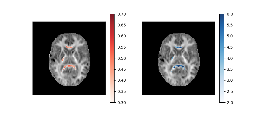

Axonal water fraction (left panel) and tortuosity (right panel) values of well-aligned fiber regions overlaid on a top of a mean kurtosis all-brain image.
References
Fieremans E, Jensen JH, Helpern JA (2011). White matter characterization with diffusion kurtosis imaging. NeuroImage 58: 177-188
Fieremans E, Jensen JH, Helpern JA, Kim S, Grossman RI, Inglese M, Novikov DS. (2012). Diffusion distinguishes between axonal loss and demyelination in brain white matter. Proceedings of the 20th Annual Meeting of the International Society for Magnetic Resonance Medicine; Melbourne, Australia. May 5-11.
Fieremans, E., Benitez, A., Jensen, J.H., Falangola, M.F., Tabesh, A., Deardorff, R.L., Spampinato, M.V., Babb, J.S., Novikov, D.S., Ferris, S.H., Helpern, J.A., 2013. Novel white matter tract integrity metrics sensitive to Alzheimer disease progression. AJNR Am. J. Neuroradiol. 34(11), 2105-2112. doi: 10.3174/ajnr.A3553
Hansen, B, Jespersen, SN (2016). Data for evaluation of fast kurtosis strategies, b-value optimization and exploration of diffusion MRI contrast. Scientific Data 3: 160072 doi:10.1038/sdata.2016.72
Total running time of the script: ( 3 minutes 27.683 seconds)